DMR Approach and Interpretation
DMRichR leverages the statistical algorithms from
dmrseq and bsseq, which enable the inference
of differentially methylated regions (DMRs). In these smoothing based
approaches, CpG sites with higher coverage are given a higher weight and
are used to infer the methylation level of neighboring CpGs with lower
coverage. This approach favors a larger sample size over a deeper
sequencing depth, and focuses on the differences in methylation levels
between groups, rather than the absolute levels within a group.
Together, these methodologies enable a low-pass WGBS approach (1-5x
coverage) that also works well with higher coverage datasets.
The main statistical approach applied by DMRichR::DM.R()
is dmrseq::dmrseq(), which identifies DMRs in a two step
approach:
- DMR Detection: The differences in CpG methylation for the effect of interest are pooled and smoothed to give CpG sites with higher coverage a higher weight, and candidate DMRs with a difference between groups are assembled.
- Statistical Analysis: A region statistic for each DMR, which is comparable across the genome, is estimated via the application of a generalized least squares (GLS) regression model with a nested autoregressive correlated error structure for the effect of interest. Then, permutation testing of a pooled null distribution enables the identification of significant DMRs. This approach accounts for both inter-individual and inter-CpG variability across the entire genome.
The main estimate of a difference in methylation between groups is
not a fold change but rather a beta coefficient, which is representative
of the average effect
size; however, it is on the scale of the arcsine transformed
differences and must be divided by π (3.14) to be similar to the
mean methylation difference over a DMR, which is provided in the
percentDifference column. Since the testing is permutation
based, it provides empirical p-values as well as FDR corrected
q-values.
One of the key differences between dmrseq and other DMR
identification packages, like bsseq, is that
dmrseq is performing statistical testing on the DMRs
themselves rather than testing for differences in single CpGs that are
then assembled into DMRs like bsseq::dmrFinder() does. This
unique approach helps with controlling the false discovery rate and
testing the correlated nature of CpG sites in a regulatory region, while
also enabling complex experimental designs. However, since
dmrseq::dmrseq() does not provide individual smoothed
methylation values, bsseq::BSmooth() is utilized to
generate individual smoothed methylation values from the DMRs.
Therefore, while the DMRs themselves are adjusted for covariates, the
individual smoothed methylation values for these DMRs are not adjusted
for covariates.
You can also read my general summary of the drmseq approach on EpiGenie.
Example DMR
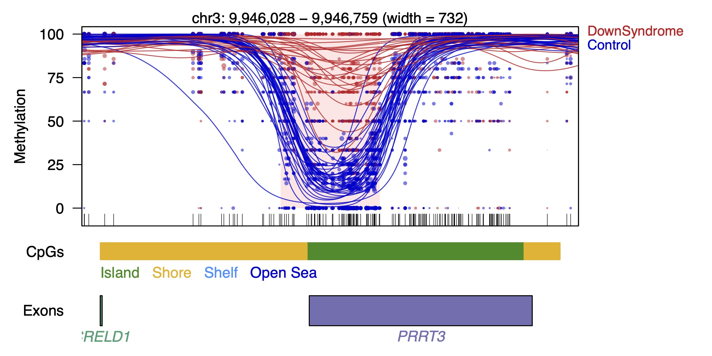 Each
dot represents the methylation level of an individual CpG in a single
sample, where the size of the dot is representative of coverage. The
lines represent smoothed methylation levels for each sample, either
control (blue) or DS (red). Gene and CpG annotations are shown below the
plot.
Each
dot represents the methylation level of an individual CpG in a single
sample, where the size of the dot is representative of coverage. The
lines represent smoothed methylation levels for each sample, either
control (blue) or DS (red). Gene and CpG annotations are shown below the
plot.
Input
Design Matrix and Covariates
This script requires a basic design matrix to identify the groups and
covariates, which should be named sample_info.xlsx and
contain header columns to identify the covariates. The first column of
this file should be the sample names and have a header labelled as
Name. In terms of the testCovariate label (i.e. Group or
Diagnosis), it is important to have the label for the experimental
samples start with a letter in the alphabet that comes after the one
used for control samples in order to obtain results for experimental
vs. control rather than control vs. experimental. You can select which
specific samples to analyze from the working directory through the
design matrix, where pattern matching of the sample name will only
select bismark cytosine report files with a matching name before the
first underscore, which also means that sample names should not contain
underscores. Within the script, covariates can be selected for
adjustment. There are two different ways to adjust for covariates:
directly adjust values or balance permutations. Overall, DMRichR
supports pairwise comparisons with a minimum of 4 samples (2 per a
group). For each discrete covariate, you should also aim to have two
samples per each grouping level.
| Name | Diagnosis | Age | Sex |
|---|---|---|---|
| SRR3537014 | Idiopathic_ASD | 14 | M |
| SRR3536981 | Control | 42 | F |
Cytosine Reports
DMRichR utilizes Bismark
cytosine reports, which are genome-wide CpG methylation count
matrices that contain all the CpGs in your genome of interest, including
CpGs that were not covered in the experiment. The genome-wide cytosine
reports contain important information for merging the top and bottom
strand of symmetric CpG sites, which is not present in Bismark
coverage and bedGraph files. In general,
cytosine reports have the following pattern:
*_bismark_bt2_pe.deduplicated.bismark.cov.gz.CpG_report.txt.gz.
CpG_Me will generate
a folder called cytosine_reports after calling the final QC
script (please don’t use the cytosine_reports_merged folder
for DMRichR). If you didn’t use CpG_Me, then you can use the
coverage2cytosine module in Bismark to
generate the cytosine reports. The cytosine reports have the following
format:
| chromosome | position | strand | count methylated | count non-methylated | C-context | trinucleotide context |
|---|---|---|---|---|---|---|
| chr2 | 10470 | + | 1 | 0 | CG | CGA |
| chr2 | 10471 | - | 0 | 0 | CG | CGG |
| chr2 | 10477 | + | 0 | 1 | CG | CGA |
| chr2 | 10478 | - | 0 | 0 | CG | CGG |
Before running the executable, ensure you have the following project directory tree structure for the cytosine reports and design matrix:
├── Project
│   ├── sample1_bismark_bt2.deduplicated.bismark.cov.gz.CpG_report.txt.gz
│   ├── sample2_bismark_bt2.deduplicated.bismark.cov.gz.CpG_report.txt.gz
│   ├── sample_info.xlsx
Running DMRichR
DMRichR::DM.R() accepts the following variables:
-
genomeSelect either: hg38, hg19, mm10, mm9, rheMac10, rheMac8, rn6, danRer11, galGal6, bosTau9, panTro6, dm6, canFam3, susScr11, TAIR10, or TAIR9. It is also possible to add other genomes withBSgenome,TxDb, andorg.dbdatabases by modifyingDMRichR::annotationDatabases(). -
coverageCpG coverage cutoff for all samples, 1x is the default and minimum value. -
perGroupPercent of samples per a group for CpG coverage cutoff, values range from 0 to 1. 0.75 (75%) is the default. -
minCpGsMinimum number of CpGs for a DMR, 5 is default. -
maxPermsNumber of permutations for the DMR analysis, 10 is default. The total number of permutations should not exceed the number of samples. -
maxBlockPermsNumber of permutations for the block analysis, 10 is default. The total number of permutations should not exceed the number of samples. -
cutoffThe cutoff value for the single CpG coefficient utilized to discover testable background regions. Values range from 0 to 1 and 0.05 (5%) is the default. If you get too many DMRs you should try 0.1 (10%). -
testCovariateCovariate to test for significant differences between experimental and control (i.e. Diagnosis). -
adjustCovariateAdjust covariates that are continuous (i.e. Age) or discrete with two or more factor groups (i.e. Sex). More than one covariate can be adjusted for (c("Sex, "Age")for R and single brackets with the;delimiter ('Sex;Age') for command line. -
matchCovariateCovariate to balance permutations, which is meant for two-group factor covariates in small sample sizes in order to prevent extremely unbalanced permutations. Only one two-group factor can be balanced (i.e. Sex). Note: This will not work for larger sample sizes (> 500,000 permutations) and is not needed for them as the odds of sampling an extremely unbalanced permutation for a covariate decreases with increasing sample size. Furthermore, we generally do not use this in our analyses, since we prefer to directly adjust for sex. -
coresThe number of cores to use, 20 is the default. The RAM requirements depend on the number of samples and coverage, which is typically between 16 to 128 GB. -
GOfuncRA logical (TRUE or FALSE) indicating whether to run a GOfuncR gene ontology analysis. This is our preferred GO method; however, it is time consuming when there is a large number of DMRs.
-
sexCheckA logical (TRUE or FALSE) indicating whether to run an analysis to confirm the sex listed in the design matrix based on the ratio of the coverage for the Y and X chromosomes. The sex chromosomes will also be removed from downstream analyses if both sexes are detected. This argument assumes there is a column in the design matrix named “Sex” [case sensitive] with Males coded as either “Male”, “male”, “M”, or “m” and Females coded as “Female”, “female”, “F”, or “f”. -
EnsDbA logical (TRUE or FALSE) indicating whether to use Ensembl transcript annotations instead of the default Bioconductor annotations, which are typically from UCSC. These annotations may allow DMRs for non-model organism genomes (i.e. rheMac10) to be mapped to substantially more genes, which will improve DMReport and gene ontology results.
R Example
DMRichR::DM.R() only requires a minimum of 2 arguments.
Your working directory should contain the contain the genome-wide
cytosine reports and design matrix.
DM.R <- function(genome = "hg38",
                 testCovariate = "Diagnosis")
However, there are total of 15 supported arguments, which have reasonable defaults:
DM.R <- function(genome = c("hg38", "hg19", "mm10", "mm9", "rheMac10",
                            "rheMac8", "rn6", "danRer11", "galGal6",
                            "bosTau9", "panTro6", "dm6", "susScr11",
                            "canFam3", "TAIR10", "TAIR9"),
                 coverage = 1,
                 perGroup =  0.75,
                 minCpGs =  5,
                 maxPerms =  10,
                 maxBlockPerms = 10,
                 cutoff = 0.05,
                 testCovariate = testCovariate,
                 adjustCovariate = NULL,
                 matchCovariate = NULL,
                 cores = 20,
                 GOfuncR = TRUE,
                 sexCheck = FALSE,
                 EnsDb = FALSE)
If your analysis contains both male and female samples, you should
adjust for sex via adjustCovariate = "Sex" and it’s highly
recommended to set sexCheck = TRUE. If you find that you’re
getting too many DMRs, you can reduce the total number by setting
cutoff = 0.1.
Command Line Example
Below is an example of how to use the executable
R script version in the exec folder on command line.
You will have to modify the path to the DM.R script in the call.
call="Rscript \
--vanilla \
/path/to/scripts/DM.R \
--genome hg38 \
--coverage 1 \
--perGroup '0.75' \
--minCpGs 5 \
--maxPerms 10 \
--maxBlockPerms 10 \
--cutoff '0.05' \
--testCovariate Diagnosis \
--adjustCovariate 'Sex;Age' \
--sexCheck TRUE \
--GOfuncR TRUE \
--EnsDb FALSE \
--cores 20"

echo $call
eval $call
UC Davis Example
If you are using the cluster at UC Davis, the following commands can
be used to execute DM.R from your login node
(i.e. epigenerate). This should be called from the working directory
that contains the cytosine reports.
module load R/3.6.3
module load homer

call="nohup \
Rscript \
--vanilla \
/share/lasallelab/programs/DMRichR/DM.R \
--genome hg38 \
--coverage 1 \
--perGroup '0.75' \
--minCpGs 5 \
--maxPerms 10 \
--maxBlockPerms 10 \
--cutoff '0.05' \
--testCovariate Diagnosis \
--adjustCovariate 'Sex;Age' \
--sexCheck TRUE \
--GOfuncR TRUE \
--cores 20 \
--EnsDb FALSE \
> DMRichR.log 2>&1 &"

echo $call
eval $call
echo $! > save_pid.txt
You can then check on the job using tail -f DMRichR.log
and ⌃ Control + c to exit the log view. You can
cancel the job from the project directory using
cat save_pid.txt | xargs kill. You can also check your
running jobs using ps -ef | grep, which should be followed
by your username i.e. ps -ef | grep blaufer. Finally, if
you still see leftover processes in htop, you can cancel all your
processes using pkill -u, which should be followed by your
username i.e. pkill -u blaufer.
Alternatively, the executable can also be submitted to the cluster
using the shell script via
sbatch DM.R.sh.
Workflow and Output
This workflow carries out the following steps:
1) Preprocess Cytosine Reports
DMRichR::processBismark() will load the genome-wide
cytosine reports, assign the metadata from the design matrix, and filter
the CpGs for equal coverage between the testCovariate as well as any
discrete adjustCovariates. There is also an option to confirm the sex of
each sample. The end result of this function is a class
bsseq object (bs.filtered) that contains the
methylated and total count data for each CpG.
2) Blocks
The bsseq object is used to identify large blocks (>
5 kb in size) of differential methylation via
dmrseq::dmrseq() by using a different smoothing approach
than the DMR calling, which “zooms out”. It will increase the minimum
CpG cutoff by 2x when compared to the DMR calling. In addition to bed
files and excel spreadsheets with the significant blocks
(sigBlocks) and background blocks (blocks),
plots of the blocks will be generated by dmrseq::plotDMRs()
and an html report with gene annotations are also generated through
DMRichR::annotateRegions() and
DMRichR::DMReport().
3) DMRs
The bsseq object is used to call DMRs through
dmrseq::dmrseq(). The DMRs typically range in size from a
several hundred bp to a few kb. In addition to bed files and excel
spreadsheets with the significant DMRs (sigRegions) and
background regions (regions), plots of the DMRs will be
generated by DMRichR::plotDMRs2() and an html report with
gene annotations are also generated through
DMRichR::annotateRegions() and
DMRichR::DMReport().
4) Smoothed Individual Methylation Values
Since dmrseq::dmrseq() smooths the differences between
groups, it isn’t possible to get individual smoothed methylation values
for downstream analyses and visualization. Therefore, the
bsseq object is smoothed using
bsseq::BSmooth() to create a new bsseq object
(bs.filtered.bsseq) with individual smoothed methylation
values.
5) ChromHMM and Reference Epigenome Enrichments
Enrichment testing from the chromHMM core 15-state
chromatin state model and the related 5 core histone modifications from
Roadmap epigenomics
127 reference epigenomes is performed using the LOLA
package through the DMRichR::chromHMM() and
DMRichR::roadmap() functions. The results are also plotted
on a heatmap by DMRichR::chromHMM_heatmap() and
DMRichR::roadmap_heatmap(). This is currently restricted to
the UC Davis cluster due to requiring large external databases; however,
an advanced user can download the
databases and modify the functions to refer to their local copy.
6) Transcription Factor Motif Enrichments
DMRichR::prepareHOMER() creates a directory with bed
files for DMRichR::HOMER() to run an enrichment analysis
for known transcription factor motifs via HOMER. Analyses will be run for
all DMRs as well for the hypermethylated and hypomethylated DMRs. The
script is set to perform the enrichment testing relative to background
regions, accommodate for percent CpG content in the normalization, and
to analyze the exact coordinates of the DMRs. The analysis will only run
if HOMER’s findMotifsGenome.pl is in the path and the
genome of interest has been installed by
configureHomer.pl.
7) Global Methylation Analyses and Plots
DMRichR::globalStats() uses the smoothed
bsseq object to test for differences in global and
chromosomal methylation with the same adjustments as the DMR calling,
where it generates an excel spreadsheet with the results and input. CpG
island statistics are also generated for almost all genomes through
through DMRichR::getCpGs(). Additionally, a number of plots
of smoothed methylation values are generated. The values for the plots
are extracted by functions that build on bsseq::getMeth().
DMRichR::windows() obtains methylation values for different
window sizes (20 Kb is the default), DMRichR::CGi() obtains
methylation values for all CpG islands, and DMRichR::CpGs()
will obtain individual CpG values. The above functions are used to
generate 3 types of plots. PCA plots are made through
DMRichR::PCA(), which uses ggbiplot. The ellipses in the
PCAs represent the 68% confidence interval, which is 1 standard
deviation from the mean for a normal distribution.
DMRichR::densityPlot() generates density plots for the mean
of each group. Finally, Glimma::glMDSPlot() is used to
generate interactive MDS plots.
8) DMR Heatmap
DMRichR::smoothPheatmap() uses
pheatmap::pheatmap() to generate a heatmap of the results
with annotations for discrete covariates. The heatmap shows the
hierarchical clustering of Z-scores for the non-adjusted percent
smoothed individual methylation values for each DMR, where the Z-score
corresponds to the number of standard deviations from the mean value of
each DMR.
9) DMR Annotations and DMRichments
DMRichR::DMRichCpG() and
DMRichR::DMRichGenic() will obtain and perform enrichment
testing for CpG and gene region (genic) annotations, respetively. The
results are plotted using DMRichR::DMRichPlot() and
DMRichR::DMparseR() enables plots with facets based on DMR
directionality. The above approach for genic annotations is similair to
what is typically preformed for arrays and other sequencing approaches,
where certain terms are given priority over others if DMRs overlap with
more than one.
10) Manhattan Plot
DMRichR::Manhattan() will take the output of
DMRichR::annotateRegions() and use it to generate a
Manhattan plot through CMplot::CMplot().
11) Gene Ontology Enrichments
Gene ontology enrichments are performed separately for all DMRs, the hypermethylated DMRs and the hypomethylated DMRs. All results all saved as excel spreadsheets. There are three approaches used, which are based on R programs that interface with widely used tools:
A) rGREAT
rGREAT enables the GREAT approach, which works for hg38, hg19, mm10, and mm9. It performs testing based on genomic coordinates and relative to the background regions. It is set to use the “oneClosest” rule.
B) GOfuncR
GOfuncR
enables the FUNC
approach, which works for all genomes and is our preferred method. It
utilizes genomic coordinates and performs permutation based enrichment
testing for the DMRs relative to the background regions, which
accommodates for gene length bias. By default,
DMRichR::GOfuncR() will only map regions to genes if they
are between 5 kb upstream and 1 downstream.
C) enrichR
enrichR enables the Enrichr approach, which is based on gene symbols and uses the closest gene to a DMR. It works for all mammalian genomes. While it doesn’t utilize genomic coordinates or background regions, it offers a number of extra databases.
rrvgo and Plots
Finally, DMRichR::slimGO() will take the significant
results from of all tools and slim them using rrvgo.
DMRichR::GOplot() will then plot the top slimmed
significant terms. This approach reduces the redundancy of closely
related terms and allows for a more comprehensive overview of the top
ontologies.
12) Machine Learning
DMRichR::methylLearn() utilizes random forest and
support vector machine algorithms from Boruta
and sigFeature
in a feature selection approach to identify the most informative DMRs
based on individual smoothed methylation values. It creates an excel
spreadsheet and an html report of the results along with a heatmap.
13) RData
The output from the main steps is saved in the RData folder so that it can be loaded for custom analyses or to resume an interrupted run:
settings.RData contains the parsed command line options
given to DMRichR as well as the annotation database variables. These
variables are needed for many of the DMRichR functions, and if you need
to reload them, you should also run
DMRichR::annotationDatabases(genome) after, since some of
the annotation databases have temporary pointers.
bismark.RData contains bs.filtered, which
is a bsseq object that contains the filtered cytosine report data and
the metadata from sample_info.xlsx in the pData.
Blocks.RData contains blocks, which is a
GRanges object of the background blocks. This can be further filtered to
produce the sigBlocks object if significant blocks are
present.
DMRs.RData contains regions and
sigRegions, which are GRanges objects with the background
regions and DMRs, respectively.
bsseq.RData contains bs.filtered.bsseq,
which is a bsseq object that has been smoothed by
bsseq::BSmooth() and is used for the individual methylation
values (but not the DMR or block calling by dmrseq, which
uses a different smoothing approach).
machineLearning.RData contains
methylLearnOutput, which is the output from the machine
learning feature selection.
Publications
The following publications utilize DMRichR:
Laufer BI*, Neier KE*, Valenzuela AE, Yasui DH, Lein PJ, LaSalle JM. Placenta and Fetal Brain Share a Neurodevelopmental Disorder DNA Methylation Profile in a Mouse Model of Prenatal PCB Exposure. Cell Reports, 2022. doi: 10.1016/j.celrep.2022.110442
Zhu Y, Gomez JA, Laufer BI, Mordaunt CE, Mouat JS, Soto DC, Dennis MY, Benke KS, Bakulski KM, Dou J, Marathe R, Jianu JM, Williams LA, Gutierrez Fugon OJ, Walker CK, Ozonoff S, Daniels J, Grosvenor LP, Volk HE, Feinberg JI, Fallin MD, Hertz-Picciotto I, Schmidt RJ, Yasui DH, LaSalle JM. Placental Methylome Reveals a 22q13.33 Brain Regulatory Gene Locus Associated with Autism. Genome Biology, 2022. doi: 10.1186/s13059-022-02613-1
Laufer BI, Hasegawa Y, Zhang Z, Hogrefe CE, Del Rosso LA, Haapanan L, Hwang H, Bauman MD, Van de Water JA, Taha AY, Slupsky CM, Golub MS, Capitanio JP, VandeVoort CA, Walker CK, LaSalle JM. Multi-omic brain and behavioral correlates of cell-free fetal DNA methylation in macaque maternal obesity models. bioRxiv preprint. doi: 10.1101/2021.08.27.457952
Brown AP, Cai L, Laufer BI, Miller LA, LaSalle JM, Ji, H. Long-term effects of wildfire smoke exposure during early life on the nasal epigenome in rhesus macaques. Environment International, 2022. doi: 10.1016/j.envint.2021.106993
Laufer BI*, Gomez JA*, Jianu JM, LaSalle, JM. Stable DNMT3L Overexpression in SH-SY5Y Neurons Recreates a Facet of the Genome-Wide Down Syndrome DNA Methylation Signature. Epigenetics & Chromatin, 2021. doi: 10.1186/s13072-021-00387-7
Maggio AG, Shu HT, Laufer BI, Hwang H, Bi C, Lai Y, LaSalle JM, Hu VW. Impact of exposures to persistent endocrine disrupting compounds on the sperm methylome in regions associated with neurodevelopmental disorders. medRxiv preprint, 2021. doi: 10.1101/2021.02.21.21252162
Mordaunt CE, Jianu JM, Laufer BI, Zhu Y, Dunaway KW, Bakulski KM, Feinberg JI, Volk HE, Lyall K, Croen LA, Newschaffer CJ, Ozonoff S, Hertz-Picciotto I, Fallin DM, Schmidt RJ, LaSalle JM. Cord blood DNA methylome in newborns later diagnosed with autism spectrum disorder reflects early dysregulation of neurodevelopmental and X-linked genes. Genome Medicine, 2020. doi: 10.1186/s13073-020-00785-8
Laufer BI, Hwang H, Jianu JM, Mordaunt CE, Korf IF, Hertz-Picciotto I, LaSalle JM. Low-Pass Whole Genome Bisulfite Sequencing of Neonatal Dried Blood Spots Identifies a Role for RUNX1 in Down Syndrome DNA Methylation Profiles. Human Molecular Genetics, 2020. doi: 10.1093/hmg/ddaa218
Murat El Houdigui S, Adam-Guillermin C, Armant O. Ionising Radiation Induces Promoter DNA Hypomethylation and Perturbs Transcriptional Activity of Genes Involved in Morphogenesis during Gastrulation in Zebrafish. International Journal of Molecular Sciences, 2020. doi: 10.3390/ijms21114014
Wöste M, Leitão E, Laurentino S, Horsthemke B, Rahmann S, Schröder C. wg-blimp: an end-to-end analysis pipeline for whole genome bisulfite sequencing data. BMC Bioinformatics, 2020. doi: 10.1186/s12859-020-3470-5
Lopez SJ, Laufer BI, Beitnere U, Berg E, Silverman JL, Segal DJ, LaSalle JM. Imprinting effects of UBE3A loss on synaptic gene networks and Wnt signaling pathways. Human Molecular Genetics, 2019. doi: 10.1093/hmg/ddz221
Vogel Ciernia A*, Laufer BI*, Hwang H, Dunaway KW, Mordaunt CE, Coulson RL, Yasui DH, LaSalle JM. Epigenomic convergence of genetic and immune risk factors in autism brain. Cerebral Cortex, 2019. doi: 10.1093/cercor/bhz115
Laufer BI, Hwang H, Vogel Ciernia A, Mordaunt CE, LaSalle JM. Whole genome bisulfite sequencing of Down syndrome brain reveals regional DNA hypermethylation and novel disease insights. Epigenetics, 2019. doi: 10.1080/15592294.2019.1609867
Acknowledgements
The development of this program was suppourted by a Canadian
Institutes of Health Research (CIHR) postdoctoral fellowship
[MFE-146824] and a CIHR
Banting postdoctoral fellowship [BPF-162684]. Hyeyeon Hwang developed
methylLearn() and the sex checker for
processBismark(). Charles Mordaunt developed
getBackground() and plotDMRs2() as well as the
CpG filtering approach in processBismark(). I would also
like to thank Keegan
Korthauer, Matt Settles,
and Ian Korf, and Janine
LaSalle for invaluable discussions related to the bioinformatic
approaches utilized in this repository.